Simulating a bark beetle outbreak in Julia

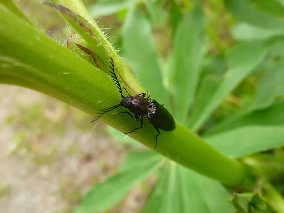
Bark beetles reproduce in the inner bark of trees. Many species attack and kill live trees. Most, however, live in dead, weakened, or dying hosts. They play a tremendous role in forest ecology - some people fear that beetles plague could annihilate even strong and healthy forests. Are those fears justified?

We will try to find the answer by modeling the bark beetle outbreak with differential equations. This post is a fragment of a study project I have done with my partner Anna Klimiuk. In the project, we generally discussed different epidemiological models, but here I will cover only the part about modeling bark beetle outbreak, including:

• implementation of Runge-Kutta 4th order method,
• a dynamical model for bark beetle outbreaks proposed here,
• numerical solution of this model,
• 2D adaptation of the model,
• 2D visualization of beetle bark outbreak on a forest map.

Also, please have in mind that this is just an insight into the project, so shortcuts are inevitable. If you have any questions, feel free to ask in the comment section.

Runge-Kutta 4th order method

This method can be applied only to ODEs in the form of

Let $h > 0$ - step height. The RK4 approximation of $y(t_{n+1}) = y_{n+1}$ is given by

where

Surprisingly, the implementation of this method in Julia is quite simple. Note that below is a vectorized version, so it can handle a system of equations and thus make it easy to solve most epidemiological models.

function vectorized_rk4_step(h, equations, values)
    k1 = h*[ eq(values...) for eq in equations ]
    k2_params = values+[h, k1...]/2 
    k2 = h*[ eq(k2_params...) for eq in equations ]
    k3_params = values+[h, k2...]/2 
    k3 = h*[ eq(k3_params...) for eq in equations ]
    k4_params = values+[h, k3...]
    k4 = h*[ eq(k4_params...) for eq in equations ]

    return values[2:end]+(k1+2*k2+2*k3+k4)/6
end

Function vectorized_rk4_step takes arguments:

• h - step height
• equations - vector of ODE equations (functions)
• values - vector of values from previous step

and it returns vector of values in the next step for every equation.

To solve a system of ODEs, let’s define a function solve_model. It takes a vector of equations, its initial values, range (time range in which solution will be obtained) and a number of steps to calculate. For every step, it calls the previous function calculating step solution and updating general solution. The solution has a form of $1 \times n \times k$ tensor, where $n$ is the number of equations and $k$ the number of steps.

function solve_model(equations, initial_values, range, steps)
    h = (range[2]-range[1])/steps
    values = [ range[1], initial_values... ]
    solution = map(x -> [x], values)
    for n in 1:steps
        timestamp = n*h
        step_solution = vectorized_rk4_step(h, equations, values)
        values = [ timestamp, step_solution... ]
        solution = [ [val..., values[key]] 
                    for (key, val) in enumerate(solution)]
    end
    return solution
end

Example usage will be shown in the next section.

The beetles

How one can model an outbreak of these little guys? They occur in forests in hundreds of thousands of individuals.

Well, there is a model, based on other epidemiological models (SIR), which has been adapted to this particular scenario - the bark beetle outbreak. It is a system of four differential equations that describe small changes in four different populations. Trees in a forest can be either bark beetle free, and thus susceptible $(S)$ to infestation or else already colonized by beetles and thus infested $(I)$. A single tree becomes infested depending on a sequence of beetle-related events. First, free-flying beetles $(B)$ have to find a tree, then settle on its surface and begin to bore through the bark. Next, these attacking beetles $(A)$ must survive host tree defenses and once they get to the cambium layer, a tree becomes infested $(I)$. The more beetles are attacking a single tree, the higher chance is to beat its defenses.

For details, please refer to this paper.

These relations lead to the following system of ODEs:

There are two functions:

• $G(S, I)$ is a function that determines the tree recruitment process. It is defined as $G(S, I) = g(K-S-I)$, where $g$ is a rate at which new trees become available to be colonized by beetles and $K$ is the environment capa
• $-d I$ - death of infested trees caused by beetles,
• $e I$ - recruitment of new beetles caused by beetle reproduction in tree bark,
• $-m B$ - death of free-flying beetles,
• $-r A$ - death of attacking beetles,
• $\lambda BS$ - finding new trees by free-flying beetles and transistion from free-flying to attacking,
• $\mu$ - migration of beetles from outside.

Numerical solution

The values of necessary parameters are based on experimental data. First, we will define them in Julia and rewrite the system of ODEs into functions.

g = 10^-3 
sigma = 1*10^-5
d = 3*10^-3 
e = 50
m = 0.05 
r = 0.1 
beta_0 = 0.03 
lambda = 0.001 
K = 900 
mi = 1000 
gamma = 65
n = 5

betaFunc(A, S) = beta_0/(1 + gamma^n*(A/S)^(-n))
GFunc(S, I) = g*(K-S-I)

dS(t, S, I, B, A) = GFunc(S, I) - sigma*S - betaFunc(A, S)*S
dI(t, S, I, B, A) = betaFunc(A, S)*S - sigma*I - d*I
dB(t, S, I, B, A) = e*I - m*B - lambda*B*S + mi
dA(t, S, I, B, A) = lambda*B*S - r*A - betaFunc(A, S)*A

To solve the model, we just plug in equations, set initial values, time range and number of steps in a previously defined function solve_model.

beetles_solution = solve_model(
  [dS, dI, dB, dA], [500, 0, 0, 0], [0, 2000], 2000
)

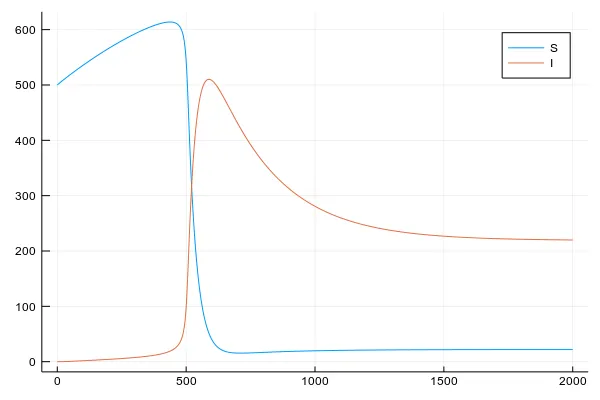
Now, plot the result.

plot(beetles_solution[1], 
  beetles_solution[2:3], label=["S" "I"]
)

plot(beetles_solution[1], 
  beetles_solution[4:5], label=["B" "A"]
)

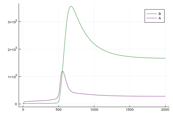
In this case, we set pretty low tree defenses parameter $\Gamma$, so once beetles accumulate into a large army, a forest gets infested in a moment. Then only newly recruited trees are healthy and there is a constant percent of infested trees. This is one of two critical points of the system. In the second one, our forest wins the battle against beetles and almost all trees remain healthy. We will see it in the 2D adaptation of this model.

2D adaptation of the model

We assume that forest can be represented as a square net in which each element is a single stand of trees. Then, we can model an interaction between those stands as

where $A, B$ are matrices representing a forest. For example $A$ may contain information about free-flying beetles and $B$ - about susceptible trees. It can be implemented in Julia as follows.

function add_zeros(M)
    # wraps a matrix M with zeros, so interact
    # function will not change a size of output matrix
    rows = size(M)[1]
    columns = size(M)[2]
    return [ zeros(1, columns+2); 
      zeros(rows, 1) M zeros(rows, 1); zeros(1, columns+2)]
end

function interact(A, B)
    A = add_zeros(A)
    B = add_zeros(B)
    return A[2:end-1, 2:end-1].*B[2:end-1, 2:end-1] + 
      A[1:end-2, 2:end-1].*B[1:end-2, 2:end-1] + 
      A[3:end, 2:end-1].*B[3:end, 2:end-1] + 
      A[2:end-1, 1:end-2].*B[2:end-1, 1:end-2] + 
      A[2:end-1, 3:end].*B[2:end-1, 3:end]
end

Using interact function we can modify some factors of our system, so beetles could spread over the square net. We apply interaction on G function as follows $G(S, I) \rightarrow \textrm{interact}\left(G(S, I), \frac{S}{\textrm{max}(S)}\right)$. Thus the forest can extend its borders and truly grow. Why $\frac{S}{\textrm{max}(S)}$? Trees can grow only in neighborhood of other trees, so we make interaction with $S$ and divide by its maximum to get only the direction of this growth multiplied by tree recruitment rate. Even more realistic model could take a minimum of this direction and some density of trees, so they won’t colonize empty stands so quickly. A similar interaction is applied to beetles migration. We assume that migration will happen from one direction and new beetles cannot magically spawn in random places, but they have to follow other beetles to discover new parts of the forest. And expression $\lambda BS$ was also transformed into interaction.

Now, we can prepare our forest. First, load a density map of some forest.

io = open("maps/forest.png", "r")
img = load(io)
img = imresize(img, ratio=1/2)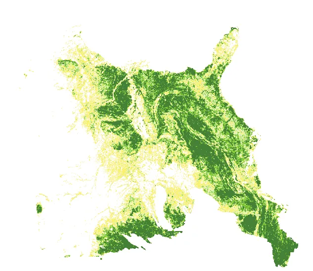

Then, convert it to black-white, scale it down and get matrices of initial values.

img_bw = Gray.(img)
S_0 = convert(Array{Float64}, img_bw)
S_0 = 1 .- S_0
# 1px is a single stand of the forest with max of K trees
S_0 = S_0.*K 

I_0 = zeros(size(S_0))
B_0 = zeros(size(S_0))
# initial beetles in the bottom right corner
B_0[end-50:end-30, end-50:end-30] .= 10 
B_0[S_0 .== 0.0] .= 0.0
A_0 = zeros(size(S_0))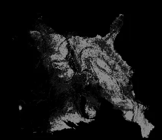

After defining all those parameters and equations again, and after slightly modifying solve_model function (now it cannot deal with matrices, but it’s just an adjustment of vectors shapes) we can obtain the solution and visualize it beautifully. Let me first present to you the final effect and then explain. This is the solution of the bark beetle outbreak in 2D.

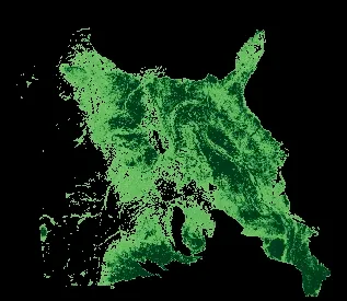
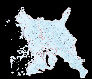
The GIF above depicts the forest and rushing wave of beetles which has its root in the bottom right corner. Red color represents attacking beetles, they colonize more and more of terrain leaving behind infested trees (blue color). Green one represents healthy trees. As you can see, this forest truly lives, it changes its shape, widens its borders. Well, we have a great visualization of the outbreak, but unfortunately, it does not tell us anything about forest condition. I created this GIF by stacking matrices of solution for $S, A, I$, thus each next layer removed some information about the previous one. And despite that those layers take different hues for different values in a matrix it is hard to say what is the final condition of the forest. We want to know a ratio of infested to healthy trees. To achieve that we will use colormap from red to blue, where blue means there is more healthy than infested trees, red means opposite, and a middle color (white) is 50-50. Then we calculate the sickness ratio for each stand of forest (each pixel) and display it using this colormap.

So, for a casual, healthy forest which has normal defense capabilities $(\Gamma = 1000)$, we and up with mostly the same, healthy forest.

For comparison, if beetles invaded already weak forest $(\Gamma = 200)$, it would have not survived.

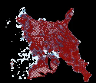
To conclude, strong and healthy forests most likely will survive such an invasion of bark beetles, but we can worry about already weak forests that are in danger.

Once again, this post was just an insight into our project, containing many shortcuts. If you want to know more details, you are welcome to ask ;)